CHAPTER 12 VCS3D Graphics Methods
Deriving actionable information from climate simulations requires the capacity to detect, compare, and analyze features spanning large heterogeneous, multi-variate, multi-dimensional datasets with spatial and temporal references. The brain’s capacity to detect visual patterns is invaluable in this knowledge discovery process. Visual mapping techniques are very effective in expressing the results of feature detection and analysis algorithms as they naturally employ the visual information processing capacity of the cerebral cortex, which is extremely difficult to emulate using statistical and machine learning approaches alone. Visual representations, which play an important role in addressing data complexity, can be enhanced by an increase in the number of “degrees of freedom” in the visual mapping process. Interactive three-dimensional views into complex high dimensional datasets can offer a widened perspective and a more comprehensive gestalt facilitating the recognition of significant features and the discovery of important patterns and relationships in the climate knowledge discovery process.
3D Plot Constituents
In the VCS model 3D perspectives are provided by the 3d_scalar and 3d_vector graphics methods. The 3d_scalar graphics method provides the Volume, Surface, and Slice display techniques (denoted henceforth as “plot constituents”). It can be used to display data in both the default (x-y-z) and Hovmoller3D (x-y-t) geometries. The 3d_vector graphics method provides the Vector slice plot constituent.
The Volume plot enables scientists to create an overview of the topology of the data, revealing complex 3D structures at a glance. It is generated using a “transfer function” to linearly map an adjustable range of variable values to an adjustable range of opacity values at each point of a 3D volume. Values of the variable that fall outside of the range are invisible (transparent). In addition, the rendered color is determined by mapping the variable’s value at each point of the volume to an adjustable range of colormap values. All three adjustable ranges can be configured either statically using a script or interactively using sliders in an active plot window.
The Surface plot can produce views similar to a volume rendering while facilitating the comparison of two variables. It is displayed as an isosurface (the higher dimensional analog of an isoline or contour line on a weather or terrain map), illustrating the surfaces of constant value for one variable and optionally colored by the spatially correspondent values of a second variable. The rendered color is determined by mapping the second variable’s value at each point of the surface to an adjustable range of colormap values. The isosurface value and the colormap range can be configured either statically using a script or interactively using sliders in an active plot window.
The Slice plot allows scientists to quickly and easily browse the 3D structure of a dataset, compare variables in 3D, and probe data values. It provides a set of three slice planes (perpendicular to the x, y, and z axes) that can be interactively dragged over the dataset. A slice through the data volume at the plane’s location is displayed by mapping the variable’s value at each point of the plane to an adjustable range of colormap values. A slice through a second data volume can also be overlaid as a contour map over the first. In an active plot window a shift-right-click on one of the planes will display the coordinates and value of the variable(s) at that point. The slice positions and the colormap range can be configured either statically using a script or interactively using sliders in an active plot window
The Vector slice plot allows scientists to browse the 3D structure of variables (such as wind velocity) that have both magnitude and direction. It provides a horizontal slice plane that can be interactively dragged over a vector field dataset (consisting of a pair of variables denoting the X and Y components of a vector at each point). A slice through the data volume at the plane’s location is displayed using a set of vector glyphs denoting the direction and magnitude of the field at a regularly spaced set of points on the plane. The slice position and the density and scaling of the vector glyphs can be configured either statically using a script or interactively using sliders in an active plot window. NOTE: this display technique can be very computationally intensive so that the higher glyph densities may cause diminished interactivity.
General 3D Plot Attributes
The 3d_scalar and 3d_vector graphics methods have the following attributes. The “expected value” is used in scripts to initialize the attribute. The attributes can also be adjusted interactively in an active plot window by clicking on the configuration button with the same name. The interaction modalities are described below for each attribute. The slider(s) appear at the bottom of the window when the attribute is being configured.
| Attribute | Use | Expected Value | Interaction Modality |
|---|---|---|---|
ToggleVolumePlot |
Toggles the visibility of the Volume (volume render) plot constituent. | vcs.on or vcs.off |
Toggle visibility with button click. |
ToggleSurfacePlot |
Toggles the visibility of the Surface (isosurface) plot constituent. | vcs.on or vcs.off |
Toggle visibility with button click. |
XSlider |
Sets the position and visibility of the Z slice plane. The position is in longitude coordinates. | ( float, vcs.on or vcs.off ) |
Adjust position with the slider. |
YSlider |
Sets the position and visibility of the Z slice plane. The position is in latitude coordinates. | ( float, vcs.on or vcs.off ) |
Adjust position with the slider. |
ZSlider |
Sets the position and visibility of the Z slice plane. The position is in relative coordinates (0.0 = bottom -> 1.0 = top). | ( float, vcs.on or vcs.off ) |
Adjust position with the slider. |
VerticalScaling |
Scales the vertical dimension of the plot. | float ~ 0.1 — 10.0 | Adjust scaling with the slider. |
ScaleColormap |
Sets the value range of the current colormap. | floats: [ max, min ]. Initialized to the max (full) value range of the data. | Adjust colormap range (min, max) with the pair of sliders. |
ScaleTransferFunction |
Sets the value range of the volume plot constituent, which maps this range of variable values to opacity. | floats: [ max, min ]. Initialized to the max (full) value range of the data. | Adjust TF range (min, max) with the pair of sliders. |
ToggleClipping |
Sets the clip bounds for the volume plot constituent. | Up to six floats: [ xmin, xmax, ymin, ymax, zmin, zmax ] | Drag the spheres on the adjustable frame. |
IsosurfaceValue |
Sets the variable value that defines the isosurface. | float between the variable max and min values. | Adjust the isosurface value using the slider. |
ScaleOpacity |
Sets the opacity range of the volume plot constituent, which maps the selected range of variable values to this opacity range. | floats: [ max, min ]. Initialized to [1,1]. | Adjust opacity range (min, max) with the pair of sliders. |
BasemapOpacity |
Sets the opacity of the underlying earth map. | float between 0.0 and 1.0. | Adjust the opacity with the slider. |
Camera |
Sets the position and orientation of the camera. | Dictionary with three keys: ‘Position’, ‘ViewUp’, and ‘FocalPoint’. The values of Position and FocalPoint are positions in model coordinates, and ViewUp is a unit vector. | Left-click in window and drag to rotate. Right-click and drag to zoom/pan. Shift-Left-click and drag to translate. |
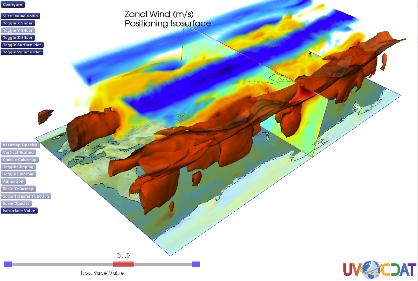
The following example illustrates these features.
Example
import vcs, cdms2, sys
x = vcs.init()
f = cdms2.open( sys.prefix+"/sample_data/geos5-sample.nc" )
v = f["uwnd"]
dv3d = vcs.get3d_scalar()
dv3d.ToggleClipping = ( 40, 360, -28, 90 )
dv3d.YSlider = ( 0.0, vcs.off )
dv3d.XSlider = ( 180.0, vcs.on )
dv3d.ZSlider = ( 0.0, vcs.on )
dv3d.ToggleVolumePlot = vcs.on
dv3d.ToggleSurfacePlot = vcs.on
dv3d.IsosurfaceValue = 31.0
dv3d.ScaleOpacity = [0.0, 1.0]
dv3d.BasemapOpacity = 0.5
dv3d.Camera = {
	'Position': (-161, -171, 279),
	'ViewUp': (.29, 0.67, 0.68),
	'FocalPoint': (146.7, 8.5, -28.6)
}
dv3d.VerticalScaling = 5.0
dv3d.ScaleColormap = ( -46.0, 48.0 )
dv3d.ScaleTransferFunction = ( 12.0, 77.0 )
x.plot( v, dv3d )
x.interact()
Resulting Plot
3D Vector Plot Attributes
The 3d_vector graphics method has the following attributes. The “expected value” is used in scripts to initialize the attribute. The attributes can also be adjusted interactively in an active plot window by clicking on the configuration button with the same name. The interaction modalities are described below for each attribute. The slider(s) appear at the bottom of the window when the attribute is being configured.
| Attribute | Use | Expected Value | Interaction Modality |
|---|---|---|---|
GlyphDensity |
Sets the spacing between the glyphs in lat/lon coordinates. | float ~ 1.0 – 20.0 | Adjust the spacing with the slider. |
GlyphSize |
Sets the glyph size scaling. | float ~ 0.1 – 1.0 | Adjust the scaling with the slider. |
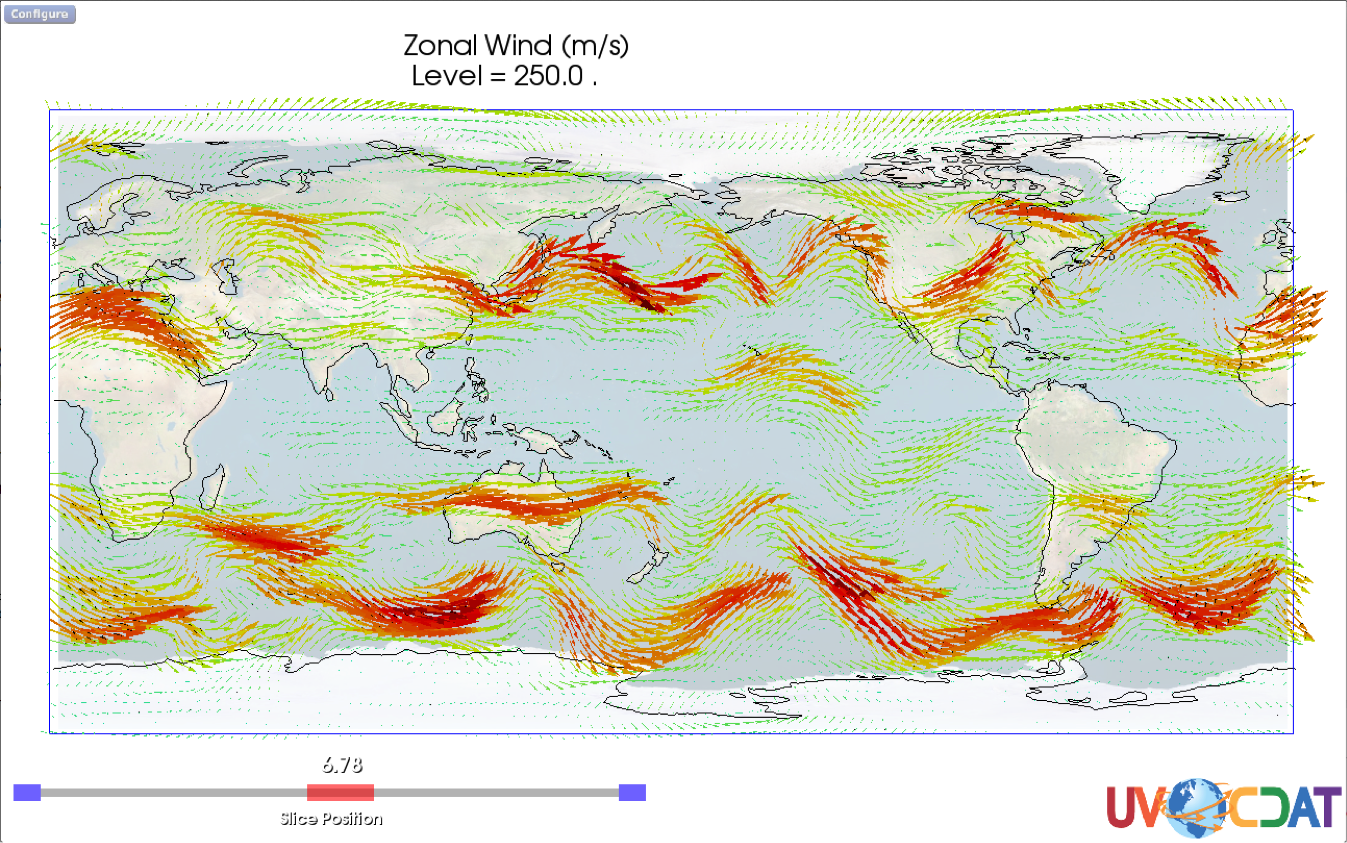
The following example illustrates these features.
Example
import vcs, cdms2, sys
x = vcs.init()
f = cdms2.open(sys.prefix+"/sample_data/geos5-sample.nc")
v = f["vwnd"]
u = f["uwnd"]
dv3d = vcs.get3d_vector()
dv3d.BasemapOpacity = 0.19
dv3d.ZSlider = 0.5
dv3d.GlyphDensity = 3.5
dv3d.GlyphSize = 0.27
x.plot( u, v, dv3d )
x.interact()
Resulting Plot
Configuring Individual Plot Constituents
The attributes illustrated above will configure all plot constituents (e.g. Volume, Surface, and Slice) simultaneously. It is also possible to configure the plot constituents separately for some graphic method attributes (currently only the scaling of opacity and colormap). This is accomplished using a dictionary with keys designating the constituents to be configured (Volume, Surface or Slice) and values representing the corresponding configurations. For example, one can use the following command to set the colormap scaling to [ 16.0, 30.0 ] for the Volume constituent, [ 30.0, 35.0 ] for the Surface constituent, and [ -46.0, 48.0 ] for all other constituents:
dv3d.ScaleColormap = ( [ -46.0, 48.0 ], { 'Volume': [ 16.0, 30.0 ], 'Surface': [ 30.0, 35.0 ] }The following example illustrates these features.
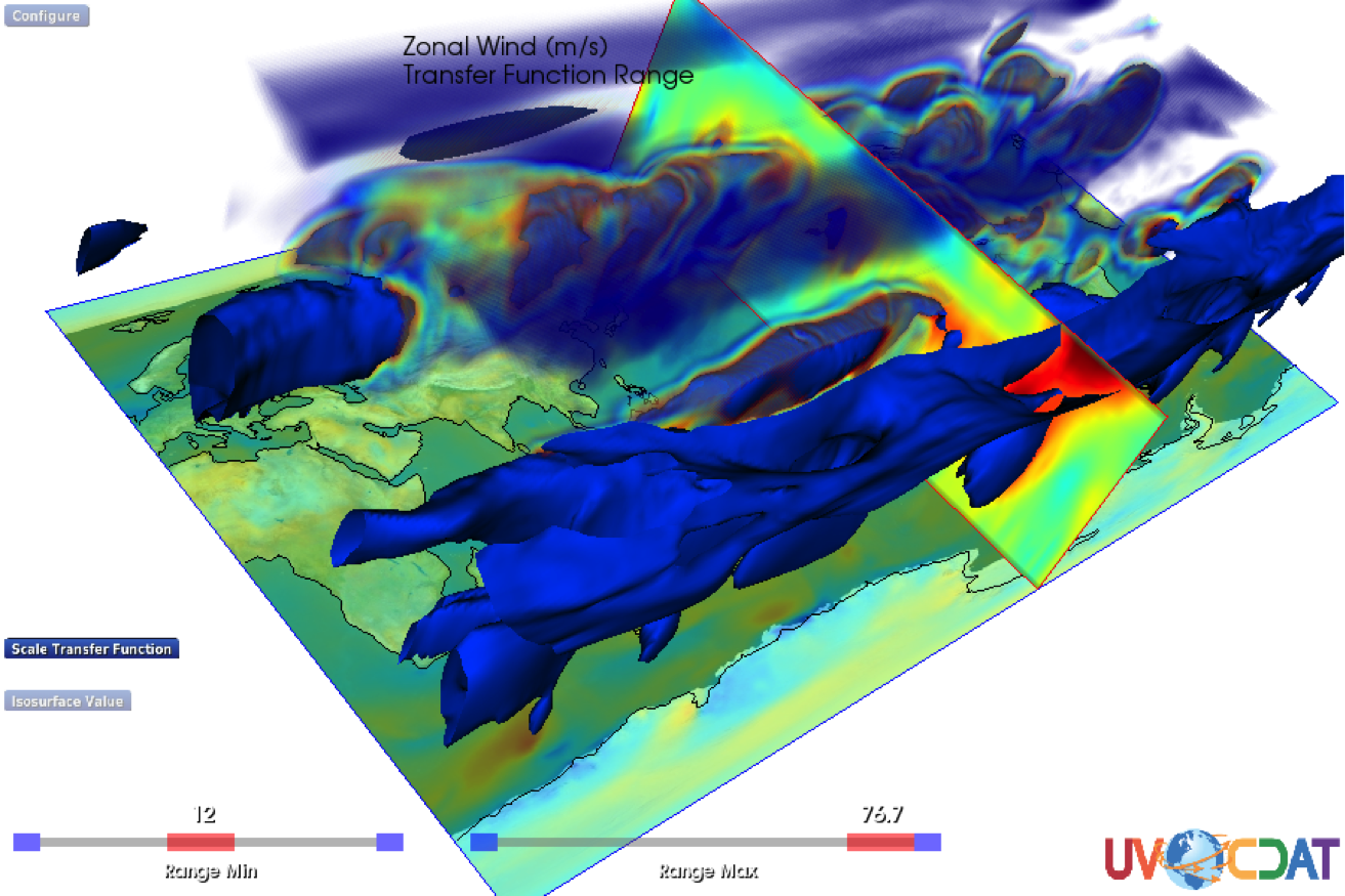
Example
import vcs, cdms2, sys
x = vcs.init()
f = cdms2.open( sys.prefix+"/sample_data/geos5-sample.nc" )
v = f["uwnd"]
dv3d = vcs.get3d_scalar()
dv3d.ToggleClipping = ( 40, 360, -28, 90 )
dv3d.YSlider = ( 0.0, vcs.off )
dv3d.XSlider = ( 180.0, vcs.on )
dv3d.ZSlider = ( 0.0, vcs.on )
dv3d.ToggleVolumePlot = vcs.on
dv3d.ToggleSurfacePlot = vcs.on
dv3d.IsosurfaceValue = 31.0
dv3d.ScaleOpacity = { 'Volume': [0.0, 0.3] }
dv3d.BasemapOpacity = 0.5
dv3d.Camera = {
	'Position': (-161, -171, 279),
	'ViewUp': (.29, 0.67, 0.68),
	'FocalPoint': (146.7, 8.5, -28.6)
}
dv3d.VerticalScaling = 5.0
dv3d.ScaleColormap = [ -46.0, 48.0 ], { 'Volume': [ 16.0, 30.0 ], 'Surface': [ 30.0, 35.0 ] }
dv3d.ScaleTransferFunction = [ 12.0, 77.0 ]
x.plot( v, dv3d )
x.interact()
Resulting Plot
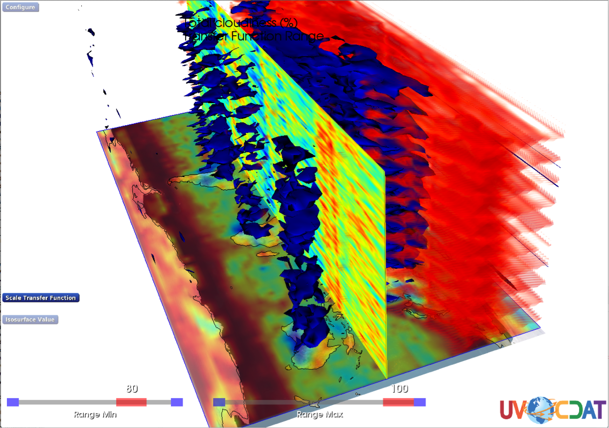
3D Hovmoller Plot
Hovmoller3D is a scalar plot that allows scientists to quickly and easily browse the 3D structure of spatial time series. It enables all of the scalar plot constituents to operate on a data volume structured with latitude and longitude in the horizontal plane and time in the vertical direction.
Example
import vcs, cdms2, sys
x = vcs.init()
f = cdms2.open(sys.prefix+"/sample_data/clt.nc")
v = f["clt"]
dv3d = vcs.get3d_scalar('Hovmoller3D')
dv3d.ToggleSurfacePlot = vcs.on
dv3d.ToggleVolumePlot = vcs.on
dv3d.IsosurfaceValue = [ 10.0 ]
dv3d.ToggleClipping = [-180.0, 175.0, -22.0, 90.0, 0.0, 119.0 ]
dv3d.ScaleTransferFunction = [80, 100, 1]
dv3d.ScaleOpacity={ 'Volume': [0.0, 0.2] }
dv3d.ZSlider = ( 0.0, vcs.on )
dv3d.YSlider = ( 20.0, vcs.on )
dv3d.Camera={'Position': (436.8, -126.3, 285.2), 'ViewUp': (-0.5, 0.25, 0.83), 'FocalPoint': (9.6, 19.9, -3.2)}

x.plot( v, dv3d )
x.interact()
Resulting Plot
Unstructured Grid Plots
The plots described in the previous sections are applied if the data is laid out on a rectangular lat-lon grid. If the data has a different structure, then vcs3D applies the more general unstructured grid plotter. This plotter makes no assumptions regarding the geometrical layout of the points- it visualizes the points directly (as a point cloud), with each point colored by the value of the variable at that location. By selectively filtering (and varying the opacity of) the points the plotter can generate slices, isosurfaces, and volume renderings. To facilitate interactivity the plotter drops into a low resolution mode during interactions and then generates a high resolution plot when the interaction is completed. The current version of the viewer has been tested with data from the following models: CAM, GEOS5, ECMWF, WRF, MMF.
Unstructured Grid Plot Attributes
The Unstructured Grid Plotter differs from the Structured Grid Plotter in that plot constituents are mutually exclusive– they can only be selected one at a time. The Unstructured Grid Plotter also adds the following additional plot attributes and takes an additional grid_file attribute to the vcs plot() method (which is used, if necessary, to specify a separate file containing the grid metadata).
| Attribute | Use | Expected Value | Interaction Modality |
|---|---|---|---|
PointSize |
Sets the sizes (in pixels) of the rendered points in low and high resolution modes. | ints~ [ 1 -> 12 ]: ( lowres_size, highres_size ) | Adjust the sizes (High and Low Resolution) with the sliders. |
SliceThickness |
Sets the thickness of the slices in model coordinates. Thicker slices contain more points. | float~ [ 0.001 -> 0.01 ]: ( lowres_thickness, highres_ thickness ) | Adjust the thicknesses (High and Low Resolution) with the sliders. This interaction is not operational when viewing a volume plot. |
ToggleSphericalProj |
Toggles between a spherical and flat earth projection. | vcs.on or vcs.off |
Toggle the projection with a button click. |
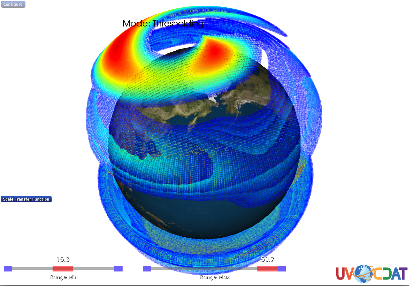
Example
x = vcs.init()
f = cdms2.open("/Data/CAM/f1850c5_t2_ANN_climo-native.nc")
v = f["U"]
dv3d = vcs.get3d_scalar()
dv3d.ToggleVolumePlot = vcs.on
dv3d.PointSize = [5, 5]
dv3d.ScaleColormap = [12.3, 33.7]
dv3d.ScaleOpacity = [0.0, 1.0]
dv3d.Camera = {'Position': (-297.2, 52.6, 340.5), 'ViewUp': (0.7, -0.15, 0.6), 'FocalPoint': (0.0, 0.0, 0.0)}
dv3d.ScaleTransferFunction = [15.3, 50.7]
dv3d.ToggleSphericalProj = vcs.on
x.plot( v, dv3d, grid_file="/Data/CAM/ne120np4_latlon.nc" )
x.interact()
Resulting Plot